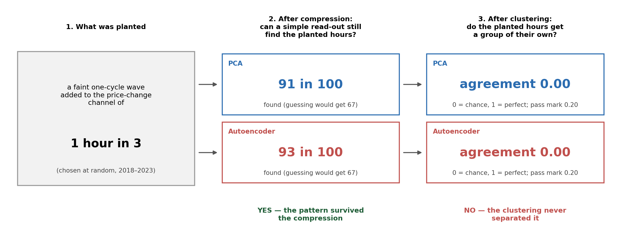
The three pipelines of the technical summary, on the real hours they were run on. Every number here is the frozen research output; the tool computes no findings of its own.
The question. Can an unsupervised pipeline discover recurring regimes in intraday US 30 price action without labels, and do they carry information about what follows? Put plainly: does a learned representation of an hour find anything more than volatility?
The answer. It finds volatility states, because volatility is what a variance-driven compression keeps; every other kind of structure planted into the data was lost or unreadable; a simpler model that could see the planted structure found no trend regime in the 2023 market beyond the clock and volatility. Data. One-minute US 30 CFD bars from Pepperstone, January 2018 to December 2023: 2.15 million overlapping 60-minute windows, 35,849 non-overlapping hours. Models are fitted on 2018–2022 and scored on 2023; calendar year 2024 is sealed. A second vendor's feed (Dukascopy) is used only to test whether clusters depend on the broker. Full method, tables and pass marks: the technical summary (PDF, 10 pages).
What happened next, by state
state definition:
Price change in the NEXT 15 minutes — mean, with 95% interval (bp)
Realised volatility of a typical hour in each state — median, with interquartile range (bp)
loading…
bp = basis points, hundredths of one percent. Bars carry the number of hours behind them. Mean and interval are the plain sample mean and ±1.96 standard errors; median and box are the plain quartiles. Computed live from the frozen hourly file: an in-sample description, not a test. The tests, with their shuffle nulls and pre-registered pass marks, are in the summary.
Pipeline 1 · linear baseline (PCA)
Each hour of 2018–2023 becomes four 60×60 pictures (Gramian angular fields), PCA squeezes the pictures to 64 numbers, and k-means sorts the hours into three groups. The question is whether the groups say anything about what price does next.
The ten experiments, in the order they were run, and where each is on this site
Benchmark check on ten labelled UCR series — passed (not shown here; in the PDF).
PCA baseline — this tab.
Autoencoder baseline — Pipeline 2.
Opening-hour test — null (in the PDF; not shown here).
Five variant configurations, each for PCA and the autoencoder — the scaling switches on this tab and Pipeline 2; the ten-out-of-ten null is in Pipeline 2's verdict.
Cross-vendor refit — technical details on this tab.
Test A, planted wave — Pipeline 2, "Why it could not do more".
Test B, planted trend followed stage by stage — Pipeline 2, same section.
Test C, direct read-out and alternative readers — Pipeline 2, the box after Test B.
Six-feature HMM benchmark — Pipeline 3.
Below: one real hour, its candles and the four pictures the pipeline received. In each picture both axes are the minutes of the hour and each pixel records how two minutes relate: red where they move alike, blue where they oppose. Click any dot on the map to load that hour here.
–
The result as a map
Two scalings were run. The baseline rescaled every hour to its own range before drawing the pictures, which discards amplitude; the V1 variant keeps one fixed scale fitted on 2018–2022. The switch below swaps between the two runs' clusters.
scaling:
colour by:
zoom:scroll wheel zooms · drag pans when zoomed · click a dot to load that hour aboveuse + / − · drag pans when zoomed · tap a dot to load that hour above
A fair sample of about 3,900 of the 2.15 million overlapping windows, placed by the frozen research output and flattened to two dimensions for display. Separation is measured in the full 64-dimensional space; this map is the illustration, not the measurement.
Verdict. With amplitude kept the three clusters are real and they last: silhouette 0.40 on the run's own sample and space (0.16 with per-window rescaling; when both models are rescored under one comparison protocol, the same 50,000 windows reduced to 64 dimensions, PCA scores 0.24 and the autoencoder 0.067, so the ranking holds), 72% of hours keep their state into the next hour where 40% would by chance, and the clusters largely coincide with a plain sort of hours into low, middle and high thirds of realised volatility (ARI 0.45). They are volatility states tied to the clock: calm (50% of hours, the Asian night, a typical realised volatility of 8 bp), thin (15%, the US lunch hour and the hour after the close, 14 bp), active (35%, the European morning and the New York session, 26 bp). On the next 15 minutes they carry nothing: η² = −0.00005 (baseline) and −0.00003 (V1) against a pre-registered pass mark of 0.06. η² is the share of the spread in next-15-minute returns accounted for by the cluster, chance-corrected, so the value random labels would reach is subtracted and noise scatters around zero, slightly negative as often as positive. One further caution: refitting the autoencoder pipeline on a second vendor's feed of the same index reproduced its clusters only weakly (ARI 0.10), so the states as found are partly a property of the broker's quote engine. Pass marks set in advance: silhouette ≥ 0.20, persistence ≥ 0.50, η² ≥ 0.06; the V1 clusters pass the first two and fail the one that matters. The check below shows the same thing on the raw hours.
Technical details
Encoding: 4-channel Gramian angular summation field over 60-bar windows of four stationary series (log return, normalised range, body ratio, causal 60-bar volume z-score). Baseline rescales each window to [−1,1]; V1 uses one scale fitted on 2018–2022.
Windows: one starts every minute (2.15 million for fitting); every test and every shuffle null is scored on one window per hour (35,849 non-overlapping hours).
Compression and grouping: incremental PCA to 64 components, L2-normalised, k-means with k from {3,5,8,12} by the gap statistic, which chose 3 in every run. Reseeding reproduces the labels (ARI 0.98); refitting the CAE pipeline on a second vendor's feed reproduces its clusters only weakly (ARI 0.10; an exploratory ablation without the tick-count channel gave 0.33).
Rule: every threshold committed before its test ran; normalisation fitted on training years only; 2024 sealed.
Pipeline 2 · deep learning (convolutional autoencoder)
The same pictures, but a convolutional autoencoder (CAE) learns the compression itself: 128 numbers per hour, trained only to rebuild the pictures. The 128 numbers are grouped with k-means exactly as in Pipeline 1, so the two are directly comparable. This was the dissertation's core method.
Put two hours side by side to see what the pictures kept and what they lost. First choose a panel, then click a dot on the map below: that hour loads into
.
Next click on the map fills the left panel.
–
–
Chart scale:
·
Under per-window rescaling those two hours produce almost the same pictures, so the size of the moves never reached the network. That is the amplitude loss described in the technical summary, and why the V1 variant keeps one fixed scale.
The result as a map
scaling:
colour by:
zoom:scroll wheel zooms · drag pans when zoomed · click a dot to load that hour aboveuse + / − · drag pans when zoomed · tap a dot to load that hour above
Verdict. The autoencoder's clusters are looser than PCA's (silhouette 0.09 with amplitude kept, 0.06 without; rescored under one protocol, 0.067 against PCA's 0.24), sort hours by the same volatility levels, and are just as silent about the next move: η² = −0.00004 (baseline) and +0.00002 (V1). Five pre-registered configurations, each run for PCA and for the autoencoder, were ten out of ten null after a family correction, the largest η² being +0.00004 against the 0.06 pass mark. The autoencoder's clusters also miss the silhouette pass mark of 0.20 that PCA's V1 clusters clear. The check below shows it on the raw hours; whether a regime could have been seen at all is answered by Pipeline 3's bound.
Why it could not do more
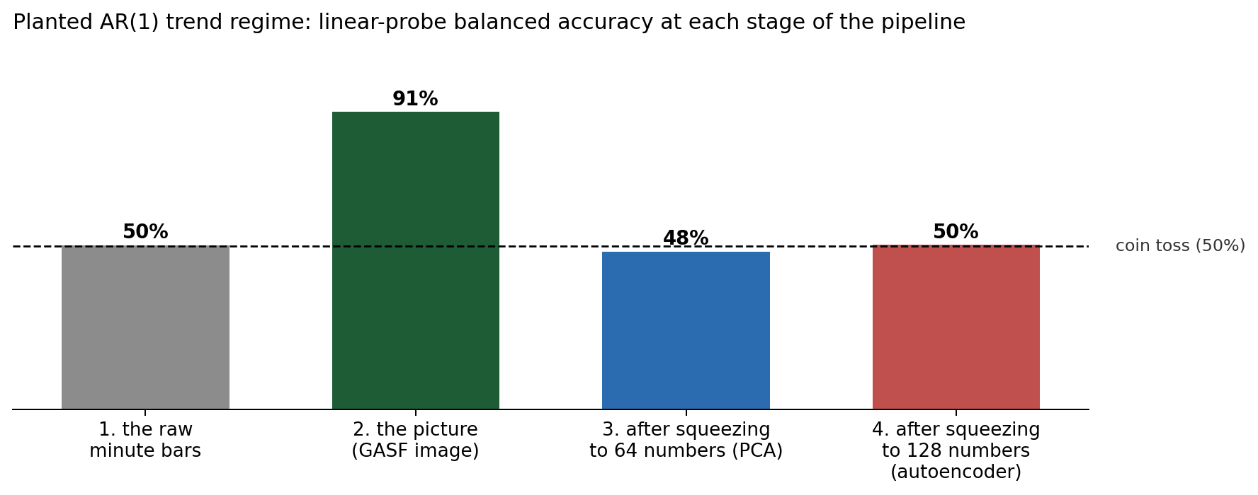
A null does not say whether a regime is absent or the pipeline cannot see one. So regimes of known strength were planted into the real inputs and followed through. The two figures are reproduced from the technical summary.
Test A: kept by the latents, discarded by the clustering. A faint wave was written into one hour in three. After compression a simple read-out could still tell planted hours from the rest (balanced accuracy of a logistic probe: 0.91 for PCA, 0.93 for the autoencoder, against 0.67 for always guessing the majority class), so the summary of each hour kept the pattern. k-means then split the hours by volatility and reported the planted group at chance (ARI 0.00) at every cluster count tried. The planted direction holds 2.7% of the latent variance; the leading volatility direction holds 17%, about six times as much, and k-means splits along the largest source of variation it can find.
Test B: where the planted trend is lost. A trend regime, each minute carrying half of the previous minute's move with the hour's total variance held fixed, was planted into one hour in three and read by a linear probe at each stage (balanced accuracy, 0.50 = chance). Unreadable in the raw bars (0.50), readable in the GASF picture (0.91), gone after PCA (0.48) and after the autoencoder (0.50). Both compressions keep what has the most variance, and a regime that leaves the variance unchanged is thrown away. A post hoc diagnostic, not pre-registered.
Asked directly, without clustering, the amplitude-kept latents predict the size of the next 15-minute move at 0.65–0.67 (balanced accuracy, small versus large, chance 0.50; the per-window baselines manage 0.51–0.52), no better than two hand-computed volatility numbers (0.67), and its direction at 0.49. On 2023 being used twice: the autoencoder's early stopping watched its reconstruction error on 2023 inputs, and the V1 scaler was fitted on inputs up to 2023, but neither ever saw a return; the probe is fitted on 2018–2022 latents and scored on 2023, and the only leakage route would be through the encoder having seen 2023 price shapes, which cannot carry the 2023 forward returns it was never shown. The clustering was not hiding a regime; there was none in the latents to hide.
Technical details
Architecture: 4×60×60 tensor → stacked 2-D convolutions → 128-d bottleneck → transposed convolutions → reconstruction, mean-squared error; early stopping on 2023 reconstruction loss (the CAE saw 2023 inputs, never returns). Latents L2-normalised before k-means.
Variants: amplitude-preserving scaling; the New York session; its first hour; 30- and 120-minute windows; each for PCA and the CAE. Family-corrected (Benjamini–Hochberg), 10/10 null.
Direct test: logistic regression fitted on the frozen 2018–2022 latents, scored on 2023; a planted wave's direction read at 0.62, so the probe is sensitive to direction when it is present.
Tests A and B showed that the compression discards a regime that does not change the variance. Pipeline 3 removes that step. Each hour is described by six hand-chosen numbers, the kind a trader looks at: how much each minute's return carries into the next one and the one after (lag-1 and lag-2 autocorrelation), how directly price travelled across the hour (path efficiency), the hour's realised volatility, the day's realised volatility, and the tick count. A Gaussian hidden Markov model, which assumes the market moves between a few hidden states that persist from hour to hour, was fitted on 2018–2022 with its number of states chosen from 4, 8 and 12 by the BIC; it chose 12, the top of the grid. Whether twelve diagonal-Gaussian states on five fit years overfit is a fair question: in 2023 the states are occupied by between 35 and 1,219 hours each, a held-out likelihood comparison across the grid was not run, and the test's answer does not rest on the choice, since the selected model explains nothing of the next hour. Each 2023 hour was then given a state from the data up to that hour only.
The states the model assigned to 2023
This is a timeline, not a picture the model sees: one thin sliver per hour of the scoring year, January on the left to December on the right, coloured by the state the HMM put that hour in. The model's only input is the six numbers above. States are numbered from the calmest (lowest median realised volatility, dark purple) to the most volatile (bright yellow). Hover for the hour; click to open it in the Any hour tab.
The test
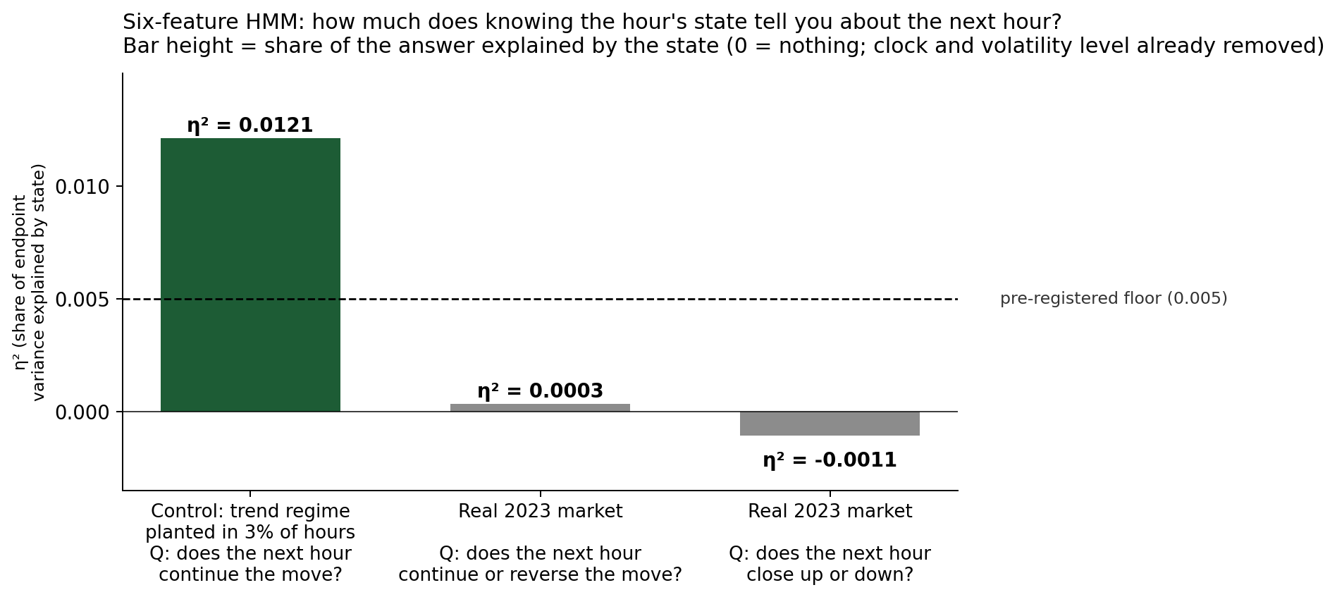
One model, three tests. Before scoring, the time of day and the volatility level were regressed out, so a state that is merely "the New York open" or "a volatile hour" earns no credit. The green bar is the model on data with a planted trend regime in 3% of hours: it found it (F1 0.72; 0.59 at 10%; pass mark F1 ≥ 0.50), and the effect cleared the pre-registered floor of 0.005 at 0.012. The grey bars are the real 2023 market, asked two different questions about the hour after a state: do minute-to-minute moves follow through or flip (trend), and does the hour as a whole close up or down (direction). Trend η² = 0.0003 with p = 0.52 under a circular-shift null; direction η² = −0.0011. A trending hour can close either way, so these are separate questions, and the model has nothing to say on either.
What the null means. Because this model recovered a planted regime at 3% prevalence, its null is a bound: the 2023 US 30 contained no persistent hour-scale trend regime at least as common as the planted ones (3% or 10% of hours) and at least as strong, once the clock and the volatility level are accounted for. A rarer or weaker regime is not excluded. The directional null is narrower, because all six features ignore the sign of moves: a regime whose only mark is that returns tend to be positive is outside this model's reach. The autoencoder's null is not a bound at all, since that pipeline never recovered a planted regime. The 2024 year was not read by any of these tests (earlier pre-registered replications read it, and each read is logged), so the null is bounded to 2023. Full detail: the technical summary (PDF).
Technical details
Model: Gaussian HMM, diagonal covariance, K from a pre-registered grid {4, 8, 12} by BIC (12 selected, the top of the grid; larger values were not pre-registered). Fitted on 2018–2022 hours; 2023 states by forward filtering. Same fit-and-score split as the direct test; no inputs or parameters shared with the CAE.
Endpoints: next-hour lag-1 autocorrelation of one-minute returns (trend / mean reversion) and next-hour signed return (direction), with hour-of-day, day-of-week and realised-volatility covariates regressed out; Kruskal–Wallis summarised by chance-corrected η²; circular-shift null of 1,000 draws; pass = BH p < 0.05 and η² ≥ 0.005 in 2023 and in the fit years.
Controls: planted trend (φ = 0.5, variance held fixed) recovered at 10% (F1 0.59) and 3% (0.72); planted wave with a directional forward effect recovered (F1 0.61); negative control at chance. The model's first feature is the statistic the trend regime was built from, so its recovery is an upper bound on what a reader can do, and the same advantage strengthens the market null.
Any hour, 2018–2023
Pick a date and a time, or arrive here from a dot on a map or a jump button. The chart shows the minute bars around that moment; the shaded band is the hour-grid window the study labelled, and the line beneath gives that hour's state under each pipeline and what price did afterwards.
–
–
Zoom:Mouse wheel zooms · drag to pan · double-click the time axis to resetPinch to zoom · drag to pan
The state labels are the frozen research outputs for the hour-grid window nearest your pick (the study cut 2018–2023 into 35,849 back-to-back hours of 60 bars). Next-15 and next-60 returns are the price change strictly after that window, in basis points. Shown for information only: none of the pipelines found the state to carry anything about the next return.